TimeSliderChoropleth#
In this example we’ll make a choropleth with a timeslider.
The class needs at least two arguments to be instantiated.
A string-serielized geojson containing all the features (i.e., the areas)
A dictionary with the following structure:
styledict = {
    '0': {
        '2017-1-1': {'color': 'ffffff', 'opacity': 1},
        '2017-1-2': {'color': 'fffff0', 'opacity': 1},
        ...
        },
    ...,
    'n': {
        '2017-1-1': {'color': 'ffffff', 'opacity': 1},
        '2017-1-2': {'color': 'fffff0', 'opacity': 1},
        ...
        }
}
In the above dictionary, the keys are the feature-ids.
Using both color and opacity gives us the ability to simultaneously visualize two features on the choropleth. I typically use color to visualize the main feature (like, average height) and opacity to visualize how many measurements were in that group.
Loading the features#
We use geopandas to load a dataset containing the boundaries of all the countries in the world.
[1]:
import geodatasets
import geopandas

datapath = geodatasets.get_path("naturalearth land")
gdf = geopandas.read_file(datapath)
Downloading file 'ne_110m_land.zip' from 'https://naciscdn.org/naturalearth/110m/physical/ne_110m_land.zip' to '/home/runner/.cache/geodatasets'.
[2]:
%matplotlib inline

ax = gdf.plot(figsize=(10, 10))
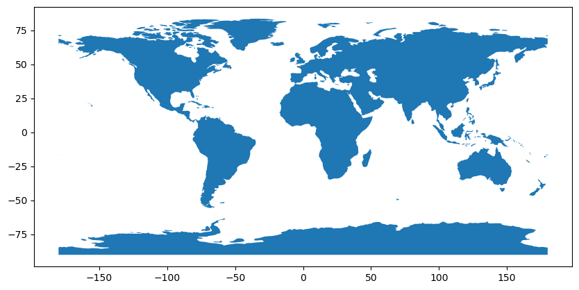
The GeoDataFrame contains the boundary coordinates, as well as some other data such as estimated population.
[3]:
gdf.head()
[3]:
| featurecla | scalerank | min_zoom | geometry | |
|---|---|---|---|---|
| 0 | Land | 1 | 1.0 | POLYGON ((-59.57209 -80.04018, -59.86585 -80.5... |
| 1 | Land | 1 | 1.0 | POLYGON ((-159.20818 -79.49706, -161.1276 -79.... |
| 2 | Land | 1 | 0.0 | POLYGON ((-45.15476 -78.04707, -43.92083 -78.4... |
| 3 | Land | 1 | 1.0 | POLYGON ((-121.21151 -73.50099, -119.91885 -73... |
| 4 | Land | 1 | 1.0 | POLYGON ((-125.55957 -73.48135, -124.03188 -73... |
Creating the style dictionary#
Now we generate time series data for each country.
Data for different areas might be sampled at different times, and TimeSliderChoropleth can deal with that. This means that there is no need to resample the data, as long as the number of datapoints isn’t too large for the browser to deal with.
To simulate that data is sampled at different times we random sample data for n_periods rows of data and then pick without replacing n_sample of those rows.
[4]:
import pandas as pd

n_periods, n_sample = 48, 40

assert n_sample < n_periods

datetime_index = pd.date_range("2016-1-1", periods=n_periods, freq="ME")
dt_index_epochs = datetime_index.astype("int64") // 10 ** 9
dt_index = dt_index_epochs.astype("U10")

dt_index
[4]:
Index(['1454198400', '1456704000', '1459382400', '1461974400', '1464652800',
       '1467244800', '1469923200', '1472601600', '1475193600', '1477872000',
       '1480464000', '1483142400', '1485820800', '1488240000', '1490918400',
       '1493510400', '1496188800', '1498780800', '1501459200', '1504137600',
       '1506729600', '1509408000', '1512000000', '1514678400', '1517356800',
       '1519776000', '1522454400', '1525046400', '1527724800', '1530316800',
       '1532995200', '1535673600', '1538265600', '1540944000', '1543536000',
       '1546214400', '1548892800', '1551312000', '1553990400', '1556582400',
       '1559260800', '1561852800', '1564531200', '1567209600', '1569801600',
       '1572480000', '1575072000', '1577750400'],
      dtype='object')
[5]:
import numpy as np

styledata = {}

for country in gdf.index:
    df = pd.DataFrame(
        {
            "color": np.random.normal(size=n_periods),
            "opacity": np.random.normal(size=n_periods),
        },
        index=dt_index,
    )
    df = df.cumsum()
    df.sample(n_sample, replace=False).sort_index()
    styledata[country] = df
Note that the geodata and random sampled data is linked through the feature_id, which is the index of the GeoDataFrame.
[6]:
gdf.loc[0]
[6]:
featurecla                                                 Land
scalerank                                                     1
min_zoom                                                    1.0
geometry      POLYGON ((-59.57209469261153 -80.0401787250963...
Name: 0, dtype: object
[7]:
styledata.get(0).head()
[7]:
| color | opacity | |
|---|---|---|
| 1454198400 | -0.444272 | -0.820469 |
| 1456704000 | -0.959682 | -0.846672 |
| 1459382400 | -2.590287 | 0.032467 |
| 1461974400 | -3.258057 | -0.039911 |
| 1464652800 | -4.263698 | -0.718590 |
We see that we generated two series of data for each country; one for color and one for opacity. Let’s plot them to see what they look like.
[8]:
ax = df.plot()
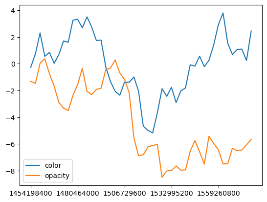
Looks random alright. We want to map the column named color to a hex color. To do this we use a normal colormap. To create the colormap, we calculate the maximum and minimum values over all the timeseries. We also need the max/min of the opacity column, so that we can map that column into a range [0,1].
[9]:
max_color, min_color, max_opacity, min_opacity = 0, 0, 0, 0

for country, data in styledata.items():
    max_color = max(max_color, data["color"].max())
    min_color = min(max_color, data["color"].min())
    max_opacity = max(max_color, data["opacity"].max())
    max_opacity = min(max_color, data["opacity"].max())
Define and apply colormaps:
[10]:
from branca.colormap import linear

cmap = linear.PuRd_09.scale(min_color, max_color)


def norm(x):
    return (x - x.min()) / (x.max() - x.min())


for country, data in styledata.items():
    data["color"] = data["color"].apply(cmap)
    data["opacity"] = norm(data["opacity"])
[11]:
styledata.get(0).head()
[11]:
| color | opacity | |
|---|---|---|
| 1454198400 | #d2b2d6ff | 0.773131 |
| 1456704000 | #d4b7d9ff | 0.769590 |
| 1459382400 | #dccae3ff | 0.888389 |
| 1461974400 | #e0d2e7ff | 0.878609 |
| 1464652800 | #e6deedff | 0.786898 |
Finally we use pd.DataFrame.to_dict() to convert each dataframe into a dictionary, and place each of these in a map from country id to data.
[12]:
styledict = {
    str(country): data.to_dict(orient="index") for country, data in styledata.items()
}
Creating the map#
[13]:
import folium
from folium.plugins import TimeSliderChoropleth


m = folium.Map([0, 0], zoom_start=2)

TimeSliderChoropleth(
    gdf.to_json(),
    styledict=styledict,
).add_to(m)

m
[13]:
Initial timestamp#
By default the timeslider starts at the beginning. You can also select another timestamp to begin with using the init_timestamp parameter. Note that it expects an index to the list of timestamps. In this example we use -1 to select the last timestamp.
[14]:
m = folium.Map([0, 0], zoom_start=2)

TimeSliderChoropleth(
    gdf.to_json(),
    styledict=styledict,
    init_timestamp=-1,
).add_to(m)

m
[14]: